The chase: data repair and logical reasoning
$$
$$
One can view the task of modeling as trying to capture a phenomenon in terms of structure (what exists) as well as properties that hold of that structure, expressed in form of logical constraints. The chase is an algorithm which enforces logical constraints that trades off well for expressivity and computational tractability. We will give a description of the algorithm at a high level, explore the language of constraints it allows us to enforce, and describe the details of its implementation in Catlab.jl. The applications below will show that this tradeoff is well-suited for tasks in scientific computing and knowledge representation.
Introduction
Let’s create a simple model of chemistry with atoms, molecules, and bonds. Atoms have a functional relationship to molecules, molecule: {\rm Atom} \rightarrow {\rm Molecule}, i.e. every {\rm Atom} relates to exactly one {\rm Molecule} (molecule can be thought of as a function from {\rm Bond} to {\rm Molecule}) . Bonds are a kind of entity that can exist between pairs of atoms. We can relate a bond to its two atoms via functional relationships bond_1, bond_2: {\rm Bond} ⟶ {\rm Atom}. If we write {b=bond(x,y)}, then implicitly we mean that there exists a bond b and atoms x and y such that bond_1(b)=x and bond_2(b)=y. Intuitively, bonds ought satisfy the following properties: - Bonds are symmetric, expressed as {∀ x,y \in {\rm Atom},\ bond(x,y) \implies bond(y,x)}. - Atoms in different molecules can’t be bonded: {\forall x,y \in {\rm Atom}, bond(x,y) \implies molecule(x) = molecule(y)}.
So far we have entities (e.g. {\rm Atom}, {\rm Bond}, {\rm Molecule}) and functional relationships (e.g. molecule). Relational databases are an ubiquitous technology that has been heavily optimized to work with data of this form. In the language of relational databases, entities are viewed as tables, with their functional relationships viewed as columns (also called foreign keys). The structure of a model that is implemented as a relational database is given by a schema which lists the entities and functional relationships. This specification of schemas is typically handled by SQL, which has been incredibly successful in many domains; however, this framework leaves something to be desired in terms of declaring and enforcing properties of our model. Ologs (ontology logs), on the other hand, are a category-theoretic interpretation of knowledge bases, which are structurally identical to relational databases yet have a rich logic of constraints that can further encode knowledge (Spivak and Kent 2012). Being able to enforce these constraints in a computationally tractable way is a difference between databases and knowledge bases.
For example: supposing we have a database of atoms, bonds, and molecules along with a set of constraints (hereafter referred to as \Sigma), we can ask whether the database satisfies \Sigma. If not, we can imagine there being the best or nearest-relative of the database that does satisfy \Sigma. The chase is an algorithm that repairs our data to find this other database (Benedikt et al. 2017). The next two sections respectively show how to define this notion of a “best” relative and describe the language in which constraints for the chase are specified.
Given a chase engine, what practical things can we do? Firstly, we have a general means of propagating information implied by the properties of a model, allowing for databases to be used as ologs. This will be described at the end of the post, along with other applications such as model enumeration (exploring logically-constrained search spaces). A future post will describe applications to e-graphs (equational reasoning that can be used for program optimization).
Data repair: defining a ‘best possible’ repaired database
In AlgebraicJulia, we represent relational databases as \mathsf{C}-sets.1 \mathsf{C}-set homomorphisms (also called morphisms) are a natural relation to consider between two \mathsf{C}-sets with the same schema. In the special cases of \mathsf{C}-sets that correspond to the categories of sets and directed graphs, the notion of a \mathsf{C}-set homomorphism lines up precisely with the notions of function and graph homomorphism, respectively. Viewing \mathsf{C}-sets as databases, these morphisms also correspond to database homomorphisms as studied in the literature.
At a high level, a morphism I\rightarrow J is a particular way of locating I within J. If a morphism exists, it is like saying there is a match of pattern I within J, and the morphism itself contains the data for how to locate I. Elements of I may be merged together when located within J, but connections may never be split apart. Consider the following visualizations of two \mathsf{C}-sets with schema {\rm Bond} \overset{b_1}{\underset{b_2}{\rightrightarrows}} {\rm Atom} \xrightarrow{mol} {\rm Molecule}.2
using Catlab, Catlab.Theories, Catlab.CategoricalAlgebra
@present SchChem(FreeSchema) begin
(Molecule, Atom, Bond)::Ob
(b₁, b₂)::Hom(Bond, Atom)
mol::Hom(Atom, Molecule)
end
@acset_type Chem(SchChem)
# Initialize empty C-sets
c₁, c₂, monotomic, diatomic, triatomic = [Chem() for _ in 1:5]
mols = [monotomic, diatomic, triatomic]
# Create 1, 2, and 3 atom molecules
[add_part!(x, :Molecule) for x in mols]
[add_parts!(x, :Atom, i, mol=1) for (i, x) in enumerate(mols)]
add_parts!(diatomic, :Bond, 2, b₁=[1,2], b₂=[2,1])
add_parts!(triatomic, :Bond, 6, b₁=[1,2,1,3,2,3], b₂=[2,1,3,1,3,2])
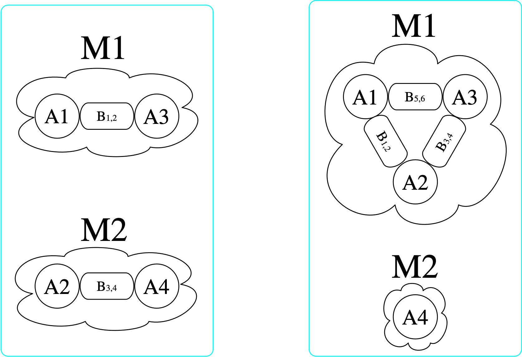
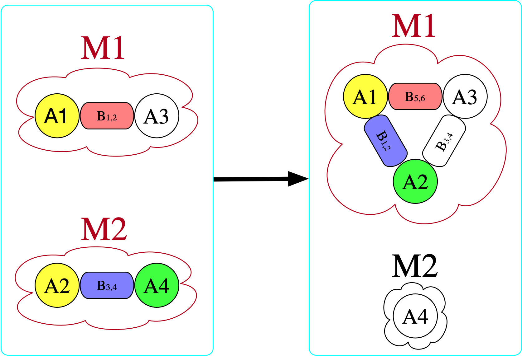
# Create the left C-set
[copy_parts!(c₁, diatomic) for _ in 1:2]
# Create the right C-set
[copy_parts!(c₂, x) for x in [triatomic, monotomic]]There are (3\cdot 2)^2=36 homomorphisms3 from the left \mathsf{C}-set (domain) to the right (codomain), one of which is indicated by coloring here:
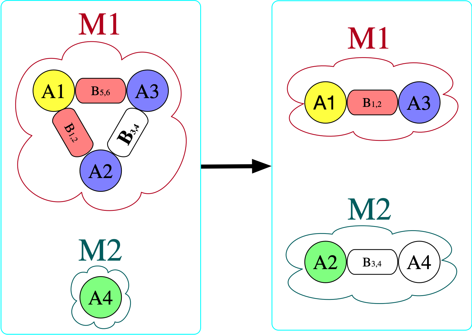
However, there is no homomorphism in the opposite direction. If we try to do this, we find that we require for there to be an atom with a bond to itself in the domain (otherwise, there is nowhere to send B₃₄ that satisfies the homomorphism constraint).
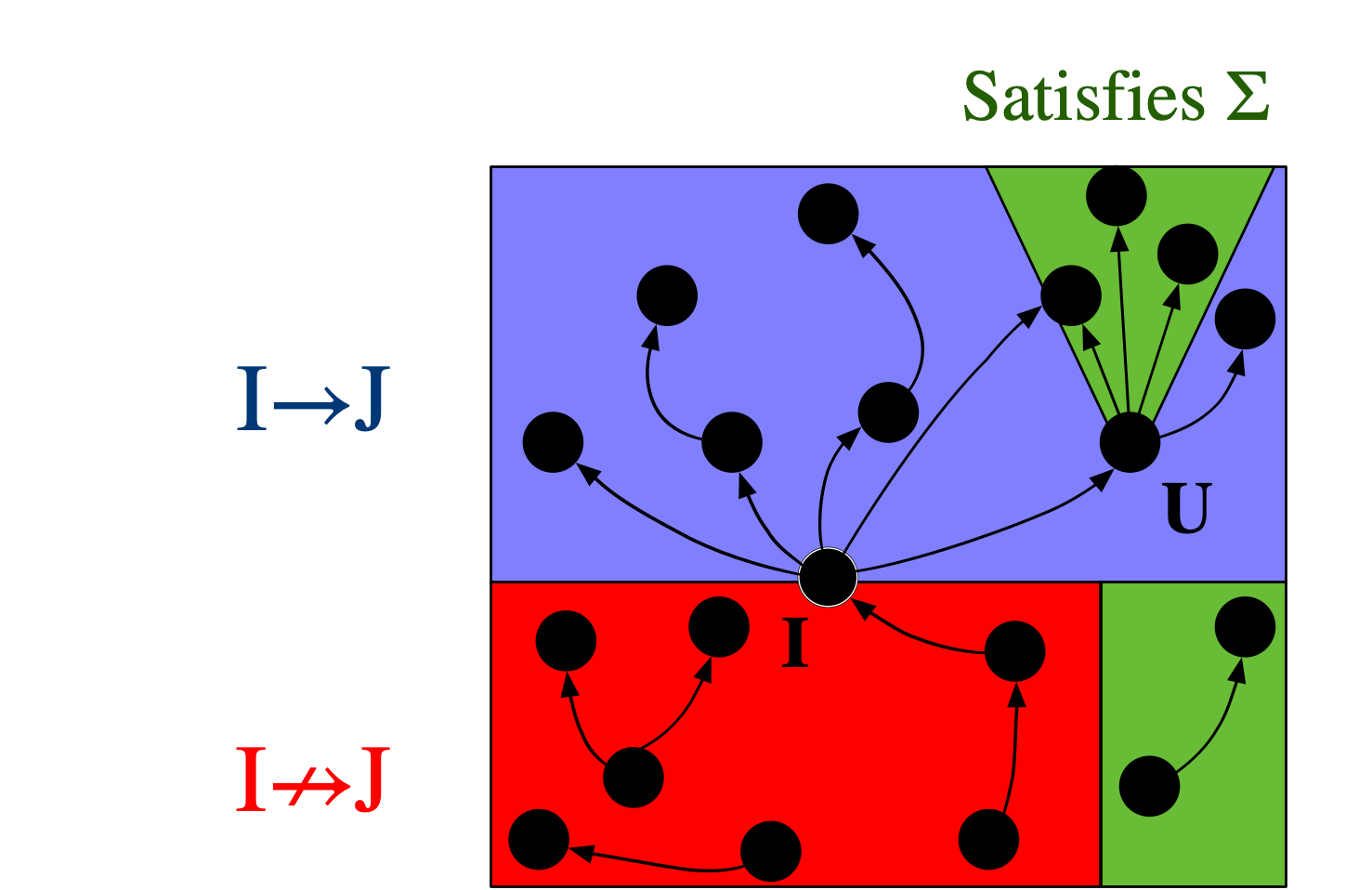
If there exists a homomorphism from I to J, one might say that I can be interpreted within J. For this reason, the binary relation I \rightarrow J (that there exists some homomorphism from I to J) is crucial in defining a notion of a “best” or “closest” \mathsf{C}-set instance, in the context of data repair: we want to consider all databases which can both interpret our starting instance (all J’s for which I \rightarrow J) as well as satisfy \Sigma. Call this set of \mathsf{C}-sets J_\Sigma. Which element U \in J_\Sigma is the universal (or best) one, if any? It would have to be one such that, for all J \in J_\Sigma, it is also the case that U \rightarrow J. Put another way, U is the minimal way of getting I to satisfy \Sigma: any modification to I to make it satisfy \Sigma will have to make at least the modifications one makes to get U.
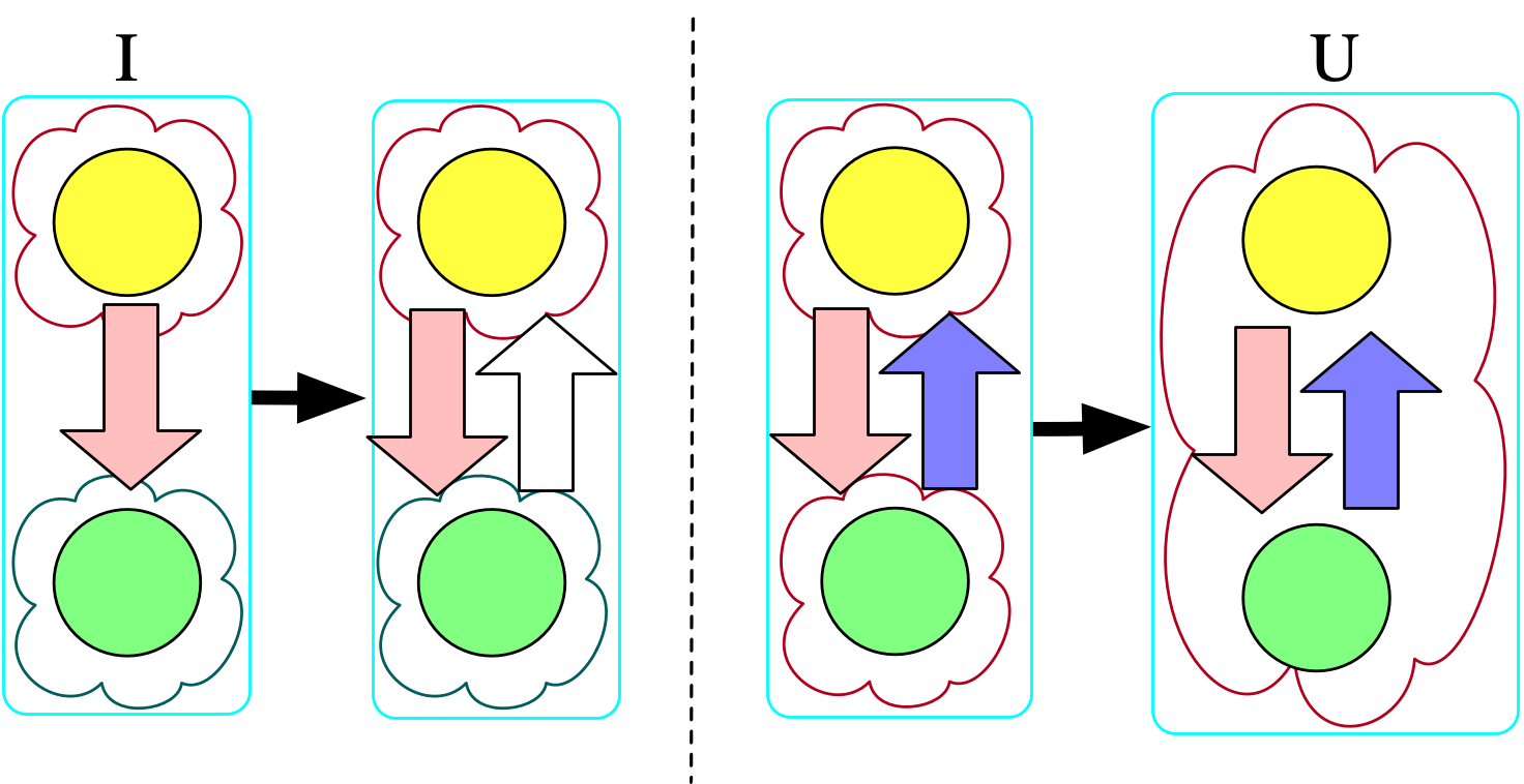
As an example, consider the instance on the far left below that doesn’t adhere to the original constraints we provided (notably, this means we must draw bonds as directed):
I = Chem()
[copy_parts!(I, monotomic) for _ in 1:2]
add_part!(I, :Bond, b₁=1, b₂=2)
@assert nparts(I, :Atom) == 2
@assert nparts(I, :Bond) == 1
@assert nparts(I, :Molecule) == 2

U = chase(I, Σ) # Σ will be described in the following section
@assert nparts(U, :Atom) == 2
@assert nparts(U, :Bond) == 2
@assert nparts(U, :Molecule) == 1
Chasing the original instance with the symmetry rule produces the first homomorphism, and then further chasing that result with our second rule (that states bonded atoms are in the same molecule) produces the second homomorphism. Although we could push further with homomorphisms (e.g. merging the two atoms together, embedding this molecule in the context of other molecules), those further transformations would not be universal with respect to the original instance and \Sigma.
Regular logic: the logic of \mathsf{C}-set homomorphisms
We cannot put arbitrary logical expressions as constraints for the chase. Rather, we are limited to expressions of the form {\forall x, \phi(x) \implies \psi(x)}, where \phi and \psi can contain \top, \land, \exists, =, and atomic formulas. This is called regular logic 4. Interestingly, these are precisely the constraints which can be encoded as homomorphisms between a source S and target T, as we have only the ability to merge things together (with =) or to add new things (with \exists), which are the restrictions we have with homomorphisms. To demonstrate this correspondance, we will show five constraints expressed as logical formulas as well as homomorphisms.
There exists at least one atom
- Our formula is: \top \implies \exists m \in {\rm Molecule}

There exists no more than one molecule
- Our formula is: \forall m_1,m_2 \in {\rm Molecule}, \top \implies m_1=m_2

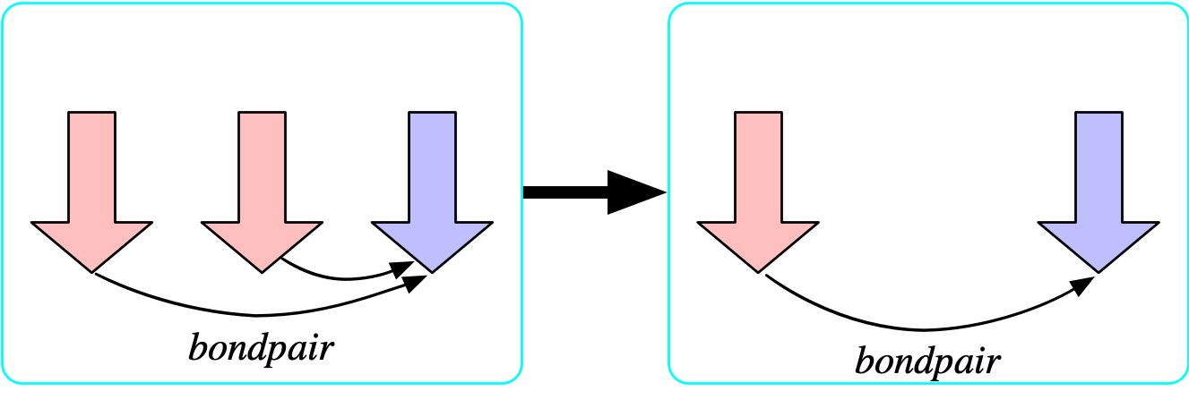
The bondpair morphism is injective
- Let us temporarily add to the schema and say there is a functional relationship {bondpair: {\rm Bond} \rightarrow {\rm Bond}} which points from any bond x \rightarrow y to its symmetric dual y\rightarrow x.
- We can prevent atoms being bonded to themselves by asserting that this is injective.
- The formula that asserts that bondpair is injective is: {\forall b_1,b_2 \in {\rm Bond}, bondpair(b_1)=bondpair(b_2) \implies b_1=b_2}
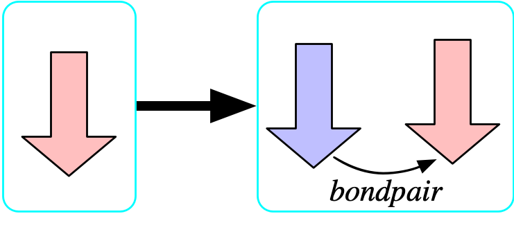
The bondpair morphism is surjective
- Our formula is: {\forall b \in {\rm Bond}, \top \implies \exists b' \in {\rm Bond},\ bondpair(b')=b}
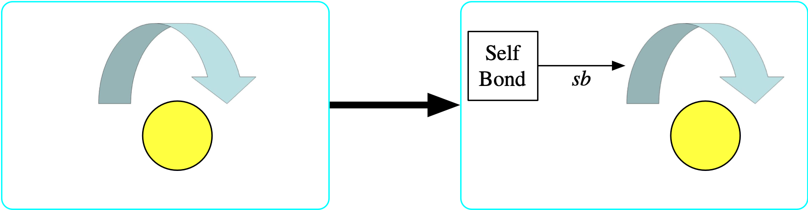
The {\rm Selfbond} object is a limit
- Again, we temporarily add to the schema an entity {\rm Selfbond} whose meaning is to identify all of the elements of {\rm Bond} that have the same source and target.
- The structure is an entity with one functional relationship sb: {\rm Selfbond} \rightarrow {\rm Bond}
- The property is \forall b \in {\rm Bond},\ bond₁(b)=bond₂(b) \implies \exists s ∈ {\rm Selfbond},\ sb(s)=b
- Visually, each element of {\rm Selfbond} will be a square and the bond that it picks out as a self bond will be indicated with an arrow labeled sb.
- Once we further constrain sb to be injective, {\rm Selfbond} becomes a limit for the diagram of a bond with the same source and target.
This correspondance is not a mere curiosity, as it has rather practical consequences. The language of the constraints can be implemented in the language of the model, so a chemist can express their knowledge in terms of molecules and atoms rather than adding a new flavor of logic to their vocabulary. More profoundly, although expressing knowledge in a logical syntax is incredibly powerful and general, this actually makes it harder to reason about and more challenging to process in an automatic way. When the same information is encoded in combinatorial (or graph-like) data, we can easily perform analyses and manipulations that are not feasible to automate for arbitrary logical formulas, mathematical expressions, or code. Some example manipulations: 1.) if the \mathsf{C} of our \mathsf{C}-sets changes because our model of the world updates, functorial data migration can faithfully migrate constraints into our new perspective when they are expressed as morphisms, 2.) the morphism representation is more clearly visualizable, further raising the accessibility and transparency of constraints as well as making a GUI for constraints possible, 3.) as will be discussed in the next section, the chase algorithm itself can be implemented in a few lines of code when thinking of constraints as morphisms, whereas it is a tedious and error-prone process to implement when working with the syntax of logical formulas.
Mathematical specification: how the chase works
In the database literature, logical constraints are known as “embedded dependencies” (EDs). Viewed as homomorphisms S \rightarrow T, each ED’s domain S is thought of as a potential trigger: it is a pattern that, if matched, obligates us to do something in order to be consistent with the constraint (either merging elements together or adding new elements). If the work to be done has not yet been done, we call the trigger active. At a high level, then, the chase merely scans for triggers, and ‘fires’ the active triggers to update the database. This process continues iteratively until there are no active triggers, if it terminates at all.
One strategy for computing the chase derives from Quillen’s small object argument, which is a general strategy for solving lifting problems, of which the chase is a special case. Given a trigger S \rightarrow I, whether or not it is active depends on whether or not there exists a homomorphism T\rightarrow I that makes the following triangle commute:
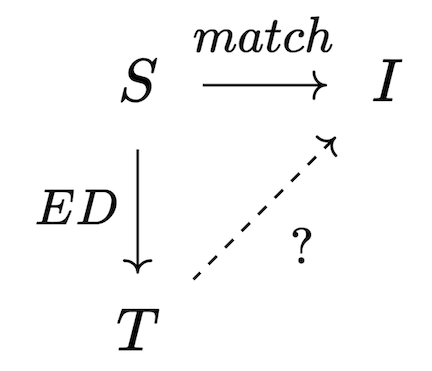
Our goal is to make the triangle commute and assume no more than necessary to make this happen; this corresponds to a categorical operation called a pushout, which produces the best possible I' for which the trigger will no longer be active; however, the new material in I' may have activated other triggers which then need to be fired. Thus, the chase can be implemented as an iteration of chase steps, each of which has the following sequence: 1. Compute all triggers of all dependencies, filtering the inactive triggers 2. Terminate the chase, if no triggers are active. 3. Construct maps from union of active triggers into the current database instance as well as into the union of trigger codomains. 4. Construct the next database instance via pushout.
Pushouts are a type of colimit that generalize unions of sets, providing a notion of “gluing pieces together along a common interface”. In this case, the interface is the top left corner of the square, which is used to connect the current database to the consequents of all triggers that fired in order to yield the next iteration of the database.
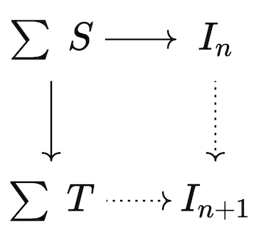
Given Catlab’s preexisting implementations for homomorphism finding and colimits, the code required to implement the chase matches closely to the mathematics.
Applications
Ologs
In scientific practice, data is usually recorded, whereas knowledge that ties data together and contextualizes it is consistently represented only informally through documentation, publications, file names, or within the behavior of obscure code. Ologs are a model of explicit knowledge representation that can be viewed in many ways (as database schemas, as ontologies, as categories). It is worthwhile to consider the pros and cons of adding formality to one’s knowledge representation. Cons are generally related to the tedium of constructing and maintaining the representation over time, whereas the pros are related to the sorts of knowledge-based tasks that can be automated in virtue of the formalization.
For example, we ask questions such as “Which reactions in my reaction network rapidly produce some molecule with a carboxyl group, according to all of the simulation software we’ve tested so far?”. How do we represent the procedure which retrieves this information? A benefit of formally-structured knowledge is that this this procedure can be written in a declarative query language, which is much more interpretable than the alternative if the data were informally distributed throughout a file system. In that case, the ‘query’ would likely be an imperative function in a scripting language - this is adequate only when limited to personal use and low-complexity scenarios.
Let’s consider a specific example that extends the schema of molecules we saw earlier into a much larger olog of simulations of chemical kinetics. Below the dotted line we give examples of elements that might live in the sets corresponding to each type in the schema. The internal triangles and squares all happen to commute, emphasized by the green checkmarks.
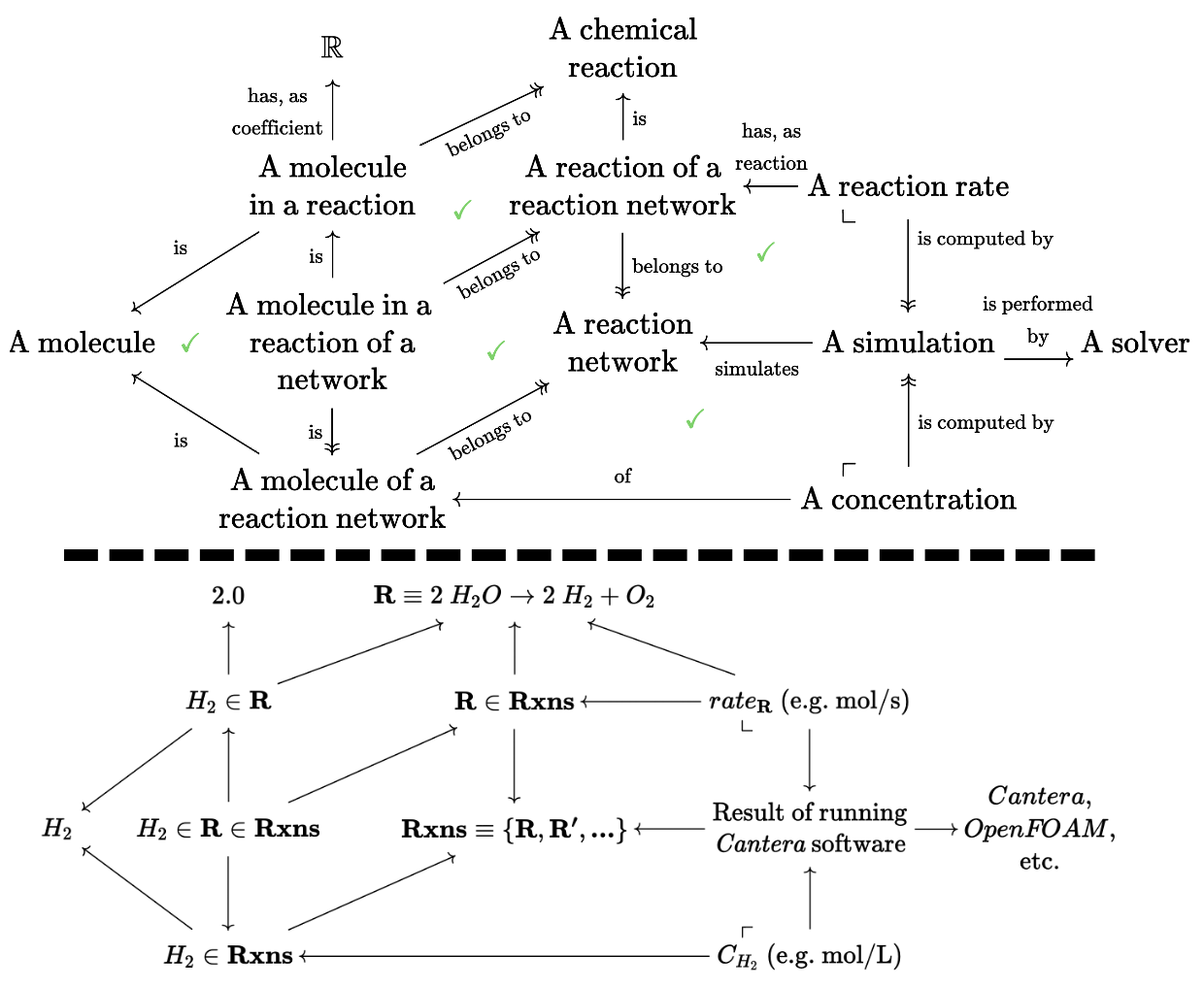
Many subtle distinctions were made at the discretion of the author of this olog, such as H_2 considered as a part of a particular reaction (has a well-defined coefficient, but doesn’t have a well-defined concentration) vs H_2 considered as a species that appears somewhere in a chemical reaction network that has been simulated (well-defined concentration, no well-defined coefficient).
The pullback constraint in the upper right corner insists that there is precisely one reaction rate corresponding to each pair of a simulation and reaction that appears in that simulation. More complicated constraints can be built from these building blocks, and the explicit (i.e. machine enforceable, via the chase as described above) nature of these constraints is powerful. This means that if one were to add a new simulation for reaction network Rxns, we can automatically add elements to the reaction rate table with their foreign keys correctly filled out. It also means we can be automatically notified of a conflict if there are two reaction rates for the same reaction and simulation pair.
Here, the chase is alleviating the general formalized knowledge problem of a scientist who is afraid to interact with their model out of fear of invalidating some subtle or intricate assumptions. As AlgebraicJulia continues to build tools to facilitate working with categories and leveraging them for scientific computing, the pros of formalization become stronger and cons become weaker.
Model enumeration
Model enumeration computes queries of the form “Show me all Petri nets up to such-and-such size” or “Show me all molecules up to such-and-such size”. This can be difficult when there are many equations at play: enumerating all groups of order 10 is difficult if we want to be more efficient than filtering a list with 10^{100} possible binary functions (after all, there are only two such groups, D_{10} and C_{10}). Why might we be interested in such queries? - Gaining evidence for a conjecture by showing it holds for all cases up to a fixed size. - Finding a counterexample in the context of property-based software test suites - Gaining intuition of complex structures through their simplest nontrivial examples. (e.g. the five simplest Kan extensions) - Exploring scientific model spaces: finding a model that best fits some data within a logically-constrained space.
By modifying one aspect of the chase, we can obtain an algorithm for model enumeration. In order for the instance U that the chase computes to be universal, when functional relationships force us to introduce a new object, it must be completely unconstrained. For example, if we fire an ED that introduces a new {\rm Bond}, then the fact that b_1,b_2 are functional relationships to {\rm Atom} means that there are two additional atoms that must be added, too. Normally, we pick fresh IDs for these atoms ((n+1, n+2), if there are n atoms already). During model enumeration, we can also consider (n+1)^2 other possibilities, where we try all \{(i,j)\ |\ 1 \leq i,j \leq n+1\}. Some of these new choices will not satisfy the axioms we seek to satisfy, but future chase steps will work towards correcting these. Ultimately, although we are searching through a combinatorial space of \mathsf{C}-sets (which are merely premodels with no notion of EDs), the fact we are using the chase to navigate this space allows us to spend effort finding models rather than enumerating the much larger set of premodels.
| Semigroup order | 1 | 2 | 3 | 4 | 5 |
|---|---|---|---|---|---|
| # of binary operations | 1 | 16 | 19,683 | 4.3×10⁹ | 3.0×10¹⁷ |
| # of semigroups | 1 | 8 | 113 | 3,492 | 183,732 |
| # of semigroups (up to isomorphism) | 1 | 5 | 24 | 188 | 1,915 |
| # of \mathsf{C}-sets explored to enumerate them all | 1 | 7 | 399 | 6,420 | 109,151 |
This preliminary data from our unoptimized prototype implementation shows that search space of possible \mathsf{C}-sets can be massively pruned using this modified chase. Being able to work with \mathsf{C}-sets up to isomorphism is essential for this strategy to avoid duplicating work.
Conclusion
Regular logic is both a computationally simple and yet expressive subset of first order logic. It is deeply connected to \mathsf{C}-set homomorphisms, allowing us to perform the chase in a broad array of modeling settings and to represent properties of our models as transparent combinatorial data.
Many scientists do not presently work with formal representations for their models of their domain, opting for a mix of text files, Python scripts, and spreadsheets distributed through a filesystem, only linked into a coherent whole within the mind of the scientist. This can be convenient for the individual, but, at a larger scale, science benefits from these models being explicit. This can be challenging work, thus there is no incentive for scientists to do this without tooling that allows individuals to reap benefits from this work investment. An important step along this path involves allowing scientists to take their formally-stated properties computationally and make them tractable to enforce.
References
Footnotes
Databases with attributes, such as
StringforFloat-valued columns, are represented as attributed \mathsf{C}-sets. These are not covered in this post.↩︎Because these bonds are symmetric, for brevity we can visually represent them as undirected.↩︎
{\rm Atom} 1 has three choices where to go (it is forced to go to {\rm Molecule} 1 in the codomain) and for each of these choices, there are two choices for {\rm Atom} 3. Each molecule in the domain is matched independently, thus the total number of morphisms will be the square of matching a single molecule.↩︎
This has limitations: we do not have the ability to state that bonds must occur between different atoms: {\forall b \in {\rm Bond},\ bond_1(b) \ne bond_2(b)}. Beyond inequalities, disjunctions are also not directly expressible. There is a computational justification for this limitation: if two things are not equal, it isn’t clear which one needs to change (and what it should change to). Likewise, if we merely know we must assign a value of x or y to something, we don’t have a straightforward automatic procedure that can pick which one we should use.↩︎